
Hello, long time no see!
This time I come here with a study case I worked on in order to finish my Google Data Analytics Professional Certificate (yay!). I spent about 4 months studying in the course, which touches a lot on the basics of analysis and of important tools like R and SQL. I’m still not a true ace on them, but I’d say I can handle myself!
This post will be a bit different from the previous ones, as I want to show how I did each phase that Google asked me to go through, from creating the business problem to presenting the insights.
Now, let’s check the case of Cyclistic Bike-Share.
The Case
You are a junior data analyst working in the marketing analyst team at Cyclistic, a bike-share company in Chicago. The director of marketing believes the company’s future success depends on maximizing the number of annual memberships. Therefore, your team wants to understand how casual riders and annual members use Cyclistic bikes differently. From these insights, your team will design a new marketing strategy to convert casual riders into annual members. But first, Cyclistic executives must approve your recommendations, so they must be backed up with compelling data insights and professional data visualizations.
Data Analysis Process
1. Ask

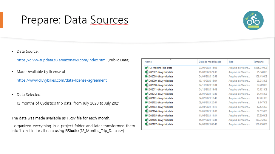
2. Prepare
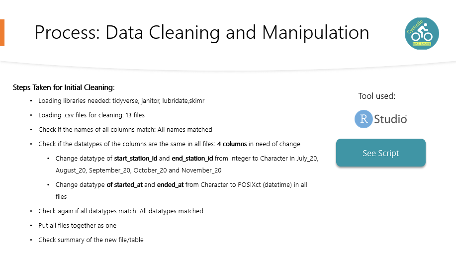
3. Process
R code follows, my observations of each step are marked with #:
#--------------------------------------------------------#
#Cleaning
#--------------------------------------------------------#

setwd("C:/Users/Glauce/Desktop/Udemy Cursos/Google Certificate/Bases_Case_Bike/Trip_Data_2020_2021")

library("tidyverse")
library("janitor")
library("lubridate")
library("skimr")

#load the datasets

july_20 <- read.csv("202007-divvy-tripdata.csv")
august_20 <- read.csv("202008-divvy-tripdata.csv")
september_20 <- read.csv("202009-divvy-tripdata.csv")
october_20 <- read.csv("202010-divvy-tripdata.csv")
november_20 <- read.csv("202011-divvy-tripdata.csv")
december_20 <- read.csv("202012-divvy-tripdata.csv")
january_21 <- read.csv("202101-divvy-tripdata.csv")
february_21 <- read.csv("202102-divvy-tripdata.csv")
march_21 <- read.csv("202103-divvy-tripdata.csv")
april_21 <- read.csv("202104-divvy-tripdata.csv")
may_21 <- read.csv("202105-divvy-tripdata.csv")
june_21 <- read.csv("202106-divvy-tripdata.csv")
july_21 <- read.csv("202107-divvy-tripdata.csv")


#check if the columns have the same name

colnames(july_20)
colnames(august_20)
colnames(september_20)
colnames(october_20)
colnames(november_20)
colnames(december_20)
colnames(january_21)
colnames(february_21)
colnames(march_21)
colnames(april_21)
colnames(may_21)
colnames(june_21)
colnames(july_21)

#All columns names match
#Check data types

compare_df_cols(july_20,
                august_20,
                september_20,
                october_20,
                november_20,
                december_20,
                january_21,
                february_21,
                march_21,
                april_21,
                may_21,
                june_21,
                july_21, return = "mismatch")

# Columns start_station_id and end_station_id have are CHR and INT, have to fix

# Also, the date fields need to be on date format

july_20 <- mutate(july_20,start_station_id = as.character(start_station_id), end_station_id = as.character(end_station_id),started_at = as.POSIXct(started_at),ended_at = as.POSIXct(ended_at))
august_20 <- mutate(august_20,start_station_id = as.character(start_station_id), end_station_id = as.character(end_station_id),started_at = as.POSIXct(started_at),ended_at = as.POSIXct(ended_at))
september_20 <- mutate(september_20,start_station_id = as.character(start_station_id), end_station_id = as.character(end_station_id),started_at = as.POSIXct(started_at),ended_at = as.POSIXct(ended_at))
october_20 <- mutate(october_20,start_station_id = as.character(start_station_id), end_station_id = as.character(end_station_id),started_at = as.POSIXct(started_at),ended_at = as.POSIXct(ended_at))
november_20 <- mutate(november_20,start_station_id = as.character(start_station_id), end_station_id = as.character(end_station_id),started_at = as.POSIXct(started_at),ended_at = as.POSIXct(ended_at))
december_20 <- mutate(december_20,started_at = as.POSIXct(started_at),ended_at = as.POSIXct(ended_at))
january_21 <- mutate(january_21,started_at = as.POSIXct(started_at),ended_at = as.POSIXct(ended_at))
february_21 <- mutate(february_21,started_at = as.POSIXct(started_at),ended_at = as.POSIXct(ended_at))
march_21 <- mutate(march_21,started_at = as.POSIXct(started_at),ended_at = as.POSIXct(ended_at))
april_21 <- mutate(april_21,started_at = as.POSIXct(started_at),ended_at = as.POSIXct(ended_at))
may_21 <- mutate(may_21,started_at = as.POSIXct(started_at),ended_at = as.POSIXct(ended_at))
june_21 <- mutate(june_21,started_at = as.POSIXct(started_at),ended_at = as.POSIXct(ended_at))
july_21 <- mutate(july_21,started_at = as.POSIXct(started_at),ended_at = as.POSIXct(ended_at))

# Check again

compare_df_cols(july_20,
                august_20,
                september_20,
                october_20,
                november_20,
                december_20,
                january_21,
                february_21,
                march_21,
                april_21,
                may_21,
                june_21,
                july_21, return = "mismatch")

#All good, no mismatches

#Time to put them together

july20_july21 <- bind_rows(july_20,
                           august_20,
                           september_20,
                           october_20,
                           november_20,
                           december_20,
                           january_21,
                           february_21,
                           march_21,
                           april_21,
                           may_21,
                           june_21,
                           july_21)

#Remove columns that are not updated for a while, according to documentation

july20_july21 <- july20_july21 %>% select(-c("start_lat", "start_lng", "end_lat", "end_lng"))

#Check the new table

head(july20_july21) #first entries

str(july20_july21) #data types

nrow(july20_july21) #number of rows

summary(july20_july21) #a numerical summary

skim(july20_july21) #summary of the columns

#Creating some columns to see year, month, day and day of the week in separate

july20_july21$month <- format(as.Date(july20_july21$started_at), "%m")
july20_july21$day <- format(as.Date(july20_july21$started_at), "%d")
july20_july21$year <- format(as.Date(july20_july21$started_at), "%Y")
july20_july21$day_of_week <- format(as.Date(july20_july21$started_at), "%A")

#Check if the new columns were placed correctly

head(july20_july21) #first entries

#Add a calculation for the length of each ride

july20_july21$ride_length <- difftime(july20_july21$ended_at,july20_july21$started_at)

#Check the new column ride_length

str(july20_july21)

#Clean rows where the bikes were just being tested (documentation states it's on HQ QR) and the rides lengths <= 0

trips_0720_0721 <- july20_july21[!(july20_july21$start_station_name == "HQ QR" | july20_july21$ride_length<=0),]

nrow(trips_0720_0721) #About 10.000 rows deleted


#---------------------------------------------------#
#Analysis
#---------------------------------------------------#

#Checking  mean, max and min values

mean(trips_0720_0721$ride_length) #1558.43 secs
max(trips_0720_0721$ride_length) #3356649 secs
min(trips_0720_0721$ride_length) #1 sec

#Checking mean, max and min by type of user

aggregate(trips_0720_0721$ride_length~trips_0720_0721$member_casual,FUN = mean)
#Casual = 2363 secs (aprox)
#member = 901 secs (aprox)

aggregate(trips_0720_0721$ride_length~trips_0720_0721$member_casual,FUN = max)
#Casual = 3356649 secs (aprox)
#member = 2005282 secs (aprox)

aggregate(trips_0720_0721$ride_length~trips_0720_0721$member_casual,FUN = min)
#Casual = 1 secs (aprox)
#member = 1 secs (aprox)

aggregate(trips_0720_0721$ride_length~trips_0720_0721$member_casual + trips_0720_0721$day_of_week,FUN = mean)
#Casual = longest on sunday, shortest on wednesday
#member = longes on sunday, shortest on thursday

july20_july21$day_of_week <- ordered(july20_july21$day_of_week, levels=c("domingo", "segunda-feira", "terça-feira", "quarta-feira", "quinta-feira", "sexta-feira", "sábado"))

aggregate(trips_0720_0721$ride_length~trips_0720_0721$member_casual + trips_0720_0721$day_of_week,FUN = mean)

#----------------------------------------------------#
#Saving
#----------------------------------------------------#

#Write .csv file

write.csv(july20_july21,"12_Months_Trip_Data.csv")
4. Analyze and 5. Share
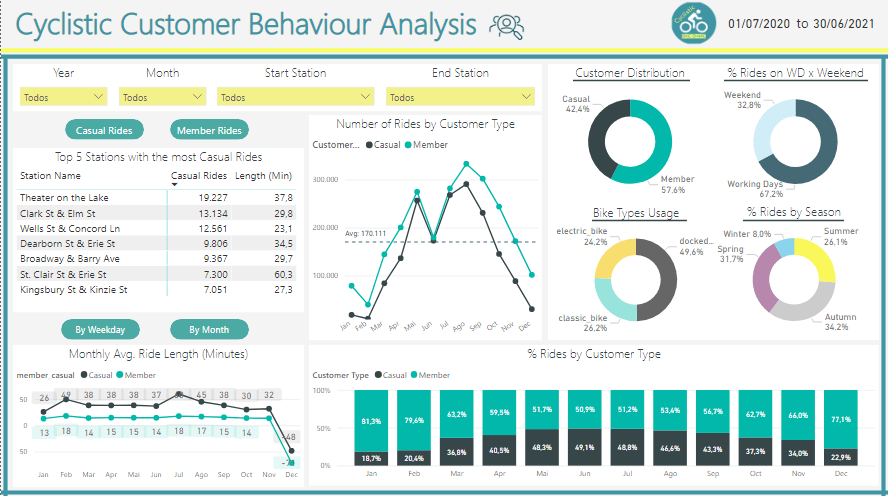
I decided to do my analysis on Power BI, as it is the tool I’m looking to improve my skills the most. After checking the data and analyzing it, the following metrics are the ones I believe makes more sense to be tracked in order to find the solutions the Marketing Team wants:
The difference between them is that clicking the green buttons lead to different table and chart on the left (Top Stations Table and Avg. Ride Length Chart).
Understanding how casual riders and annual members use Cyclistic bikes differently:
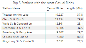
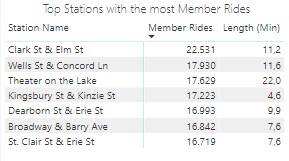
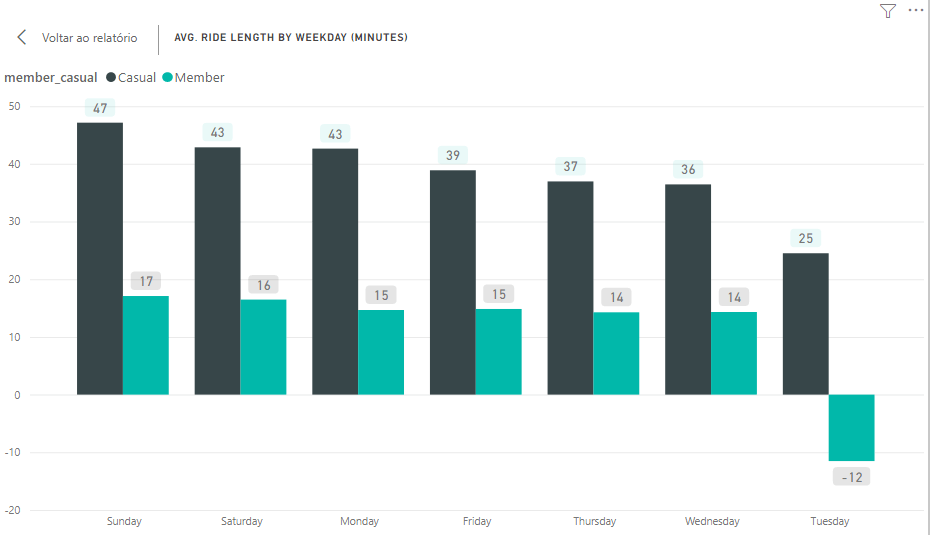
Checking on the stations with most Casual riders and most Member riders, we see basically the same names on both tables, showing these stations have a lot of movement and potential to convert Casuals into Members. Also, we see that the Casuals take longer riding the bikes, as they need to enjoy the most of each ride they pay, while the Members can ride short distances several times. This data provides some target stations for the marketing to work on, as well an argument to show Casuals why it’s more advantageous to be a member. The chart below shows better the time length difference:
Now let’s check some monthly data regards the number of rides:
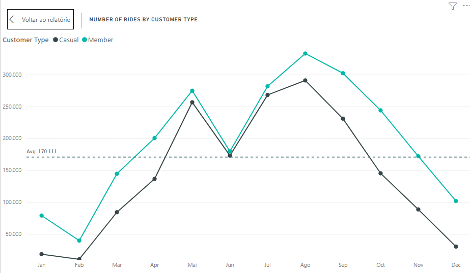
This chart gives us interesting information on the pattern of ride numbers through a year, so we see both types of customers grow and decrease their rides similarly. We also can notice that the people start riding more when spring starts (March), reaching the peak in summer (August), then they start decreasing with the start of fall (September), reaching the lowest point on February (Winter).
This piece of information can help the marketing team planning when is the best timing to run campaigns, which for sure isn’t winter.
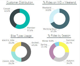
The interference of seasons can be seen on the donut chart in the bottom right, where we see about 65% of the rides happening on Spring and Autumn, when it’s not too hot or too cold.
We can also take some conclusions from the other donuts, such as:
- The ratio Casual x Member shows there is still room to grow for members % if we know how to tackle those customers;
- People ride a lot on working days, which can mean that some of those rides are not for fun but for work or other activities that can only be done on working days;
- Docked bikes are the most used by everybody.
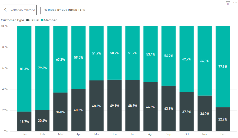
On the last chart we see the ratio Casual:Member by month, considering the number of rides. Here we see members enjoying winter and casuals coming for the service in summer.
6. Act
Recommendations
My recommendations for the marketing team would be:
- Study well some stations where they could focus the marketing campaign instead of spending resources on stations with not many casual members or potential to have changes;
- Choose to do the campaigns between May and August, which is when the ration casual:member reaches close to 50:50, making it easier for casuals to see what is being advertised;
- Focus on the Docked Bikes service, as it’s the one people use the most;
- Take in consideration that people use the service both for fun on weekends and normal life on workdays, so there can be different kinds of interest inside the casual riders group.
Conclusion
With the recommendations I close my project. If you read until here, thank you and hope you enjoyed!
I’m still far from satisfied with my knowledge, so constructive feedback is welcome. Let’s keep striving to deliver better and better insights! 🙂
